I recently resumed a dormant project, an eco-evolutionary dynamics simulation model. The model tracks biomass over time for multiple mutants and multiple species. Unsurprisingly, things broke down when I asked MATLAB to solve a series of ordinary differential equations for each morph:

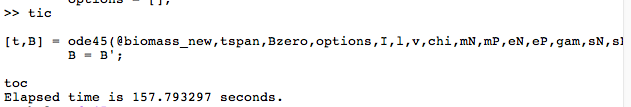
This is 157 seconds per generation of a 100,000 generation simulation. Unacceptable! Well, I accepted it for multiple runs of the simulation, but when the mutation rate was high enough, this step slows down tremendously.
I am not a trained computer scientist, but its time to optimize this code (so I can complete the simulation and publish the g-#$@% paper). After isolating this step as the inefficient problem, I went on to search for alternatives. At the moment, for a given set of conditions, this ODE solver used 344,458 time steps PER GENERATION to give a solution (for each mutant in the system).
As you can see, I chose ode45, MATLAB’s ODE workhorse. But upon further reading, I see there may be other options. Also unsurprisingly, my searching brought me to a helpful blog post by Cleve Moler over at MathWorks:
An ordinary differential equation problem is stiff if the solution being sought is varying slowly, but there are nearby solutions that vary rapidly, so the numerical method must take small steps to obtain satisfactory results.
Stiffness is an efficiency issue. If we weren’t concerned with how much time a computation takes, we wouldn’t be concerned about stiffness. Nonstiff methods can solve stiff problems; they just take a long time to do it.
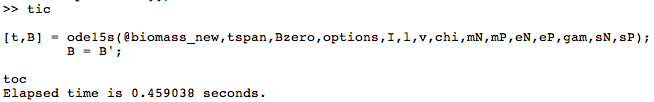
I can heartily agree that computation time led me to search for alternative solutions (HA! GET IT??) to my problem. As I gleefully change my ODE solver to MATLAB’s ode15s, which used 23 time steps to solve the same problem,
I can only (until I write the Methods section of the paper that details why I changed ODE solvers for a small set of simulation conditions or re-run the entire simulation set using this solver only) go back to Cleve to explain the difference in the solvers:
What can be done about stiff problems? You don’t want to change the differential equation or the initial conditions, so you have to change the numerical method. Methods intended to solve stiff problems efficiently do more work per step, but can take much bigger steps. Stiff methods are implicit. At each step they use MATLAB matrix operations to solve a system of simultaneous linear equations that helps predict the evolution of the solution…
Imagine you are returning from a hike in the mountains. You are in a narrow canyon with steep walls on either side. An explicit algorithm would sample the local gradient to find the descent direction. But following the gradient on either side of the trail will send you bouncing back and forth from wall to wall, as in Figure 1. You will eventually get home, but it will be long after dark before you arrive. An implicit algorithm would have you keep your eyes on the trail and anticipate where each step is taking you. It is well worth the extra concentration.
And since this blog post serves partially as my own documentation until such a time as the Methods for this paper is entirely written, permit me to quote the more dryly-put (but more precise, so dry is mighty fine for this scientist who primarily publishes in the primary literature and thus primarily values dry precision…see elsewhere in this blog for evidence of that) MATLAB help documentation:
ode45 is based on an explicit Runge-Kutta (4,5) formula, the Dormand-Prince pair. It is a one-step solver – in computing y(tn), it needs only the solution at the immediately preceding time point, y(tn-1). In general, ode45 is the best function to apply as a first try for most problems. [3]
ode15s is a variable order solver based on the numerical differentiation formulas (NDFs). Optionally, it uses the backward differentiation formulas (BDFs, also known as Gear’s method) that are usually less efficient. Like ode113, ode15s is a multistep solver. Try ode15s when ode45 fails, or is very inefficient, and you suspect that the problem is stiff, or when solving a differential-algebraic problem. [9], [10]
[3] Dormand, J. R. and P. J. Prince, “A family of embedded Runge-Kutta formulae,” J. Comp. Appl. Math., Vol. 6, 1980, pp. 19–26.
[9] Shampine, L. F. and M. W. Reichelt, “The MATLAB ODE Suite,” SIAM Journal on Scientific Computing, Vol. 18, 1997, pp. 1–22.
[10] Shampine, L. F., M. W. Reichelt, and J.A. Kierzenka, “Solving Index-1 DAEs in MATLAB and Simulink,” SIAM Review, Vol. 41, 1999, pp. 538–552.