I plan to calculate the spatial gradient of Daphnia magna traits for 20 sample sites in Belgium. The spatial gradient is inspired by Loarie et al. 2009’s The velocity of climate change. Loarie et al. (2009) simply describe their calculation of spatial gradient as:
I found more information about this average maximum technique here (its referred to explicitly as the average maximum technique here):
This is information basically for how to calculate elevation (or other) slopes as degrees or radians. I did not follow 100% of these instructions. I decided to use this average maximum technique to calculate the magnitude of the gradient in units (of trait) per meter.
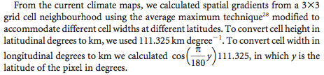
One initial question I had was why the cell width in longitudinal degrees was multiplied by cos(pi / 180 * latitude). I found this explanation:
If the two points are near each other, for example in the same city, estimating the great circle with a straight line in the latitude-longitude space will produce minimal error, and be a lot faster to calculate. A minor complication is the fact that the length of a degree of longitude depends on the latitude: a degree of longitude spans 111km on the Equator, but half of that on 60° north. Adjusting for this is easy: multiply the longitude by the cosine of the latitude. Then you can just take the Euclidean distance between the two points, and multiply by the length of a degree:
distance(lat, lng, lat0, lng0):
    deglen := 110.25
    x := lat - lat0
    y := (lng - lng0)*cos(lat0)
    return deglen*sqrt(x*x + y*y)
So basically, the size of a degree in longitude depends on what latitude it is measured for.
The next step for me was determining the distance between points in my georeferenced map of Belgium. I obtained a map of Belgium’s administrative boundaries here. One important step was creating a geotiff (a georeferenced .tif image). I loaded the shapefile BEL_adm0.shp then saved that as an image in .tif format.
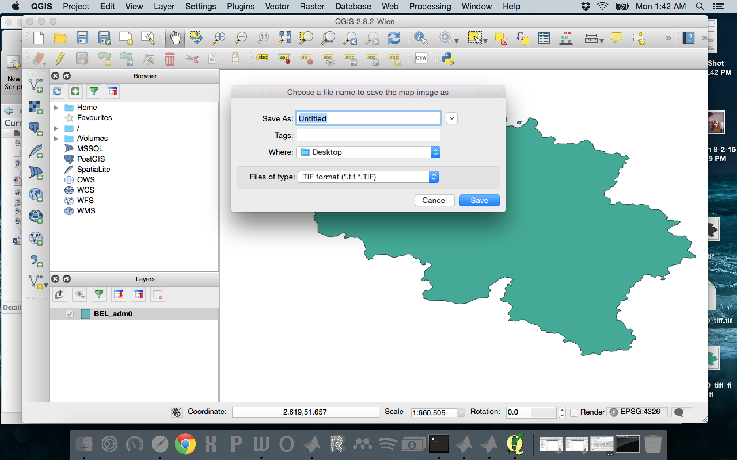
This automatically creates the .tif file and a .tifw file – the worldfile that contains the following information:
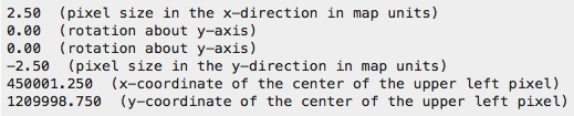
This appeared to be great news! But I realized that the image was low resolution, this instance was 578×847, and there was no way to input the desired resolution. Back to the drawing board! I then discovered its possible to set the resolution using the QGIS command line:
qgis --project myproject.qgs --snapshot image.png
            --width 1500 --height 1000 --extent xmin,ymin,xmax,ymax
In QGIS, I displayed the map of Belgium (simply the BEL_adm0.shp file) at the desired resolution (1:10,000) and saved that as a QGIS project. In Terminal, my command was:
/Applications/QGIS.app/Contents/MacOS/QGIS --project BEL.qgs --snapshot BEL.png --width 3000 --height 2000 --extent 2.46428,49.425,6.432,51.878636
(The ‘–extent’ information is the extent of the map window in latitude/longitude coordinates. These will display manually in the QGIS window if you scroll around the borders of where you want the map image to draw.)
I then created a new MATLAB file based on the information found in the MATLAB help for ‘geotiffwrite’:
basename = 'BEL';
imagefile = [basename '.png'];
RGB = imread(imagefile);
RGB_new = RGB(:,:,1);
%Derive world file name from image file name, read the world file, and construct a spatial referencing object.
worldfile = 'BEL.PNGw';
R = worldfileread(worldfile, 'geographic', size(RGB_new));
%Write image data and referencing data to GeoTIFF file.
filename = ['new' '.tif'];
geotiffwrite(filename, RGB_new, R)
If I re-read the geotiff file into MATLAB:
[A, R] = geotiffread('new.tif');
I now have R, a spatialref.GeoRasterReference object, with the following attributes (from MATLAB help documentation)
Latlim: [0.5 2.5]
Lonlim: [0.5 2.5]
RasterSize: [2 2]
RasterInterpretation: ‘cells’
AngleUnits: ‘degrees’
ColumnsStartFrom: ‘south’
RowsStartFrom: ‘west’
DeltaLat: 1
DeltaLon: 1
RasterExtentInLatitude: 1
RasterExtentInLongitude: 1
XLimIntrinsic: [0.5 2.5]
YLimIntrinsic: [0.5 2.5]
CoordinateSystemType: ‘geographic’
For the relevant specific information:
RasterInterpretation
Controls handling of raster edges. A string that equals ‘cells’ or ‘postings’.
Default: ‘cells’
DeltaLat
Change in latitude with respect to intrinsic y. Amount by which latitude increases or decreases with respect to an increase of one unit in intrinsic y. Positive when columns start from south, and negative when columns start from north. Its absolute value equals the latitude extent of a single cell, when RasterInterpretation is ‘cells’, or the latitude separation of adjacent sample points, when RasterInterpretation is ‘postings’).
Cannot be set.
DeltaLon
Change in longitude with respect to intrinsic x. Amount by which longitude increases or decreases with respect to an increase of one unit in intrinsic x. Positive when rows start from west, and negative when rows start from east. Its absolute value equals the longitude extent of a single cell, when RasterInterpretation is ‘cells’, or the longitude separation of adjacent sample points, when RasterInterpretation is ‘postings’.
Cannot be set.
The value of R for my Belgium administrative map (with the country boundaries only) are:
 Latlim: [49.3270 51.9740]
 Lonlim: [2.4643 6.4346]
 RasterSize: [2000 3000]
 RasterInterpretation: 'cells'
 AngleUnits: 'degrees'
 ColumnsStartFrom: 'north'
 RowsStartFrom: 'west'
 DeltaLat: -0.0013
 DeltaLon: 0.0013
 RasterExtentInLatitude: 2.6469
 RasterExtentInLongitude: 3.9704
 XLimIntrinsic: [0.5000 3.0005e+03]
 YLimIntrinsic: [0.5000 2.0005e+03]
 CoordinateSystemType: 'geographic'
This tells me that each point in the 2000-by-3000 matrix in the .tif file (map of Belgium image) is separated by 0.0013 degrees of longitude and -0.0013 degrees of latitude.
According to this Wikipedia entry on Decimal degrees, “The radius of the semi-major axis of the Earth at the equator is 6,378,137.0 meters[1] resulting in a circumference of 40,075,161.2 meters. The equator is divided into 360 degrees of longitude, so each degree at the equator represents 111,319.9 metres or approximately 111.32 km.”
This tells me that each degree of latitude is separated by ~144 meters (111,319.9 * 0.0013). Each degree of longitude is separated by the same distance, adjusted for the latitude of the location.
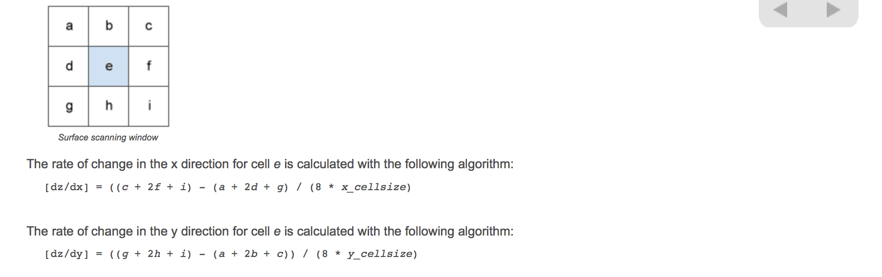
Now, to calculate the magnitude of the gradient in D. magna trait values with spatial distance, I calculate the change in the X direction and the change in Y direction using this formula:
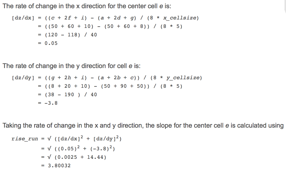
My cell width for the x direction is 0.0013(degrees)*111319.9(meters). My cell height for the y direction is 0.0013(degrees)*111319.9(meters)*cos((pi/180) * latitude of focal cell).
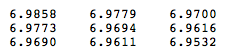
For example, for a focal and 8 neighboring cells with trait values (age at maturity, so the units are days):
I use the following formulas to get dx and dy:
map = ['a', 'b', 'c';'d', 'e', 'f';'g', 'h', 'i'];
dx = ((gradient_Tc(map=='c') + 2*gradient_Tc(map=='f') + gradient_Tc(map=='i')) - (gradient_Tc(map=='a') + 2*gradient_Tc(map=='d') + gradient_Tc(map=='g'))) / (8*R.DeltaLon*111319.9);
dy = ((gradient_Tc(map=='g') + 2*gradient_Tc(map=='h') + gradient_Tc(map=='i')) - (gradient_Tc(map=='a') + 2*gradient_Tc(map=='b') + gradient_Tc(map=='c'))) / (8*cos((pi/180)*intrinsicToGeographic(R,259,735))*111319.9*R.DeltaLon);
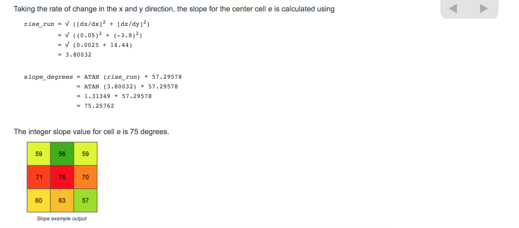
The magnitude of the gradient is the length of the hypotenuse for this triangle:
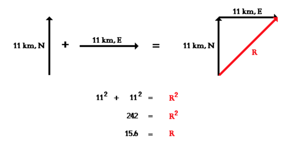
In MATLAB, I calculate:
slope = norm([dx, dy])
Giving:
dx = -5.3572e-05
dy = -9.0390e-05
slope = 1.0507e-04
So using the average maximum technique, the maximum rate of change in D. magna age at maturity from this focal cell (located at 51.001872016010672°N, 2.806393282188125°E) to its neighbors is 0.00010507 days / meter.
References
Loarie et al. 2009. The velocity of climate change. Nature 462: 1052–1055